AM–GM inequality

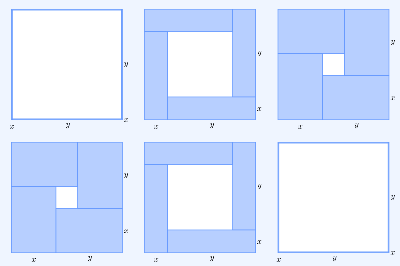
In mathematics, the inequality of arithmetic and geometric means, or more briefly the AM–GM inequality, states that the arithmetic mean of a list of non-negative real numbers is greater than or equal to the geometric mean of the same list; and further, that the two means are equal if and only if every number in the list is the same (in which case they are both that number).

The simplest non-trivial case is for two non-negative numbers and , that is,
:$\frac2 \ge \sqrt$
with equality if and only if . This follows from the fact that the square of a real number is always non-negative (greater than or equal to zero) and from the identity :
:$\begin 0 & \le (x-y)^2 \\ & = x^2-2xy+y^2 \\ & = x^2+2xy+y^2 - 4xy \\ & = (x+y)^2 - 4xy. \end$
Hence , with equality when , i.e. . The AM–GM inequality then follows from taking the positive square root of both sides and then dividing both sides by ''2''.

For a geometrical interpretation, consider a rectangle with sides of length  and ; it has perimeter and area . Similarly, a square with all sides of length has the perimeter and the same area as the rectangle. The simplest non-trivial case of the AM–GM inequality implies for the perimeters that and that only the square has the smallest perimeter amongst all rectangles of equal area.

The simplest case is implicit in Euclid's Elements, Book V, Proposition 25.

Extensions of the AM–GM inequality treat weighted means and generalized means.

Background

The ''arithmetic mean'', or less precisely the ''average'', of a list of numbers is the sum of the numbers divided by :

:$\frac.$

The ''geometric mean'' is similar, except that it is only defined for a list of ''nonnegative'' real numbers, and uses multiplication and a root in place of addition and division:

:\sqrt

If , this is equal to the exponential of the arithmetic mean of the natural logarithms of the numbers:

:$\exp \left( \frac \right).$

The inequality

Restating the inequality using mathematical notation, we have that for any list of nonnegative real numbers ,

:\frac \ge \sqrt ,,

and that equality holds if and only if .

Geometric interpretation

In two dimensions, is the perimeter of a rectangle with sides of length  and . Similarly, is the perimeter of a square with the same area, , as that rectangle. Thus for the AM–GM inequality states that a rectangle of a given area has the smallest perimeter if that rectangle is also a square.

The full inequality is an extension of this idea to dimensions. Consider an -dimensional box with edge lengths .
Every vertex of the box is connected to edges of different directions, so the average length of edges incident to the vertex is .
On the other hand, \sqrt /math> is the edge length of an -dimensional cube of equal volume, which therefore is also the average length of edges incident to a vertex of the cube.

Thus the AM–GM inequality states that only the -cube has the smallest average length of edges connected to each vertex amongst all -dimensional boxes with the same volume.

Examples

Example 1

If $a,b,c>0$, then the AM-GM inequality tells us that

:$(1+a)(1+b)(1+c)\ge 2\sqrt \cdot 2\sqrt \cdot 2\sqrt = 8\sqrt$

Example 2

A simple upper bound for $n!$ can be found. AM-GM tells us

:1+2+\dots+n \ge n\sqrt /math>

:\frac \ge n\sqrt /math>

and so

:$\left(\frac\right)^n \ge n!$

with equality at $n=1$.

Equivalently,

:$(n+1)^n \ge 2^nn!$

Example 3

Consider the function

:f(x,y,z) = \frac + \sqrt + \sqrt /math>

for all positive real numbers , and . Suppose we wish to find the minimal value of this function. It can be rewritten as:
:$\begin f(x,y,z) &= 6 \cdot \frac\\ &=6\cdot\frac \end$
with
: x_1=\frac,\qquad x_2=x_3=\frac \sqrt,\qquad x_4=x_5=x_6=\frac \sqrt

Applying the AM–GM inequality for , we get

:
\begin
f(x,y,z)
&\ge 6 \cdot \sqrt \
&= 6 \cdot \sqrt \
&= 2^ \cdot 3^.
\end

Further, we know that the two sides are equal exactly when all the terms of the mean are equal:

:f(x,y,z) = 2^ \cdot 3^ \quad \mbox \quad \frac = \frac \sqrt = \frac \sqrt

All the points satisfying these conditions lie on a half-line starting at the origin and are given by

:(x,y,z)=\biggr(t,\sqrt sqrt\,t,\frac\,t\biggr)\quad\mbox\quad t>0.

Applications

Cauchy-Schwarz inequality

The AM-GM equality can be used to prove the Cauchy–Schwarz inequality.

Annualized returns

In financial mathematics, the AM-GM inequality shows that the annualized return, the geometric mean, is less than the average annual return, the arithmetic mean.

Nonnegative polynomials

The Motzkin polynomial $x^4y^2+x^2y^4-3x^2y^2+1$ is a nonnegative polynomial which is not a sum of square polynomials. It can be proven nonnegative using the AM-GM inequality with $x_1 = x^4 y^2$, $x_2 = x^2 y^4$, and $x_3 = 1$, that is, $\le .$ Simplifying and multiplying both sides by 3 gives $\le ,$ so $.$

Proofs of the AM–GM inequality

The AM–GM inequality can be proven in many ways.

Proof using Jensen's inequality

Jensen's inequality states that the value of a concave function of an arithmetic mean is greater than or equal to the arithmetic mean of the function's values. Since the logarithm function is concave, we have

:$\log \left(\frac \right) \geq \frac \sum \log x_i = \frac \log \left( \prod x_i\right) = \log \left( \left( \prod x_i \right) ^ \right).$

Taking antilogs of the far left and far right sides, we have the AM–GM inequality.

Proof by successive replacement of elements

We have to show that

:\alpha = \frac \ge \sqrt \beta

with equality only when all numbers are equal.

If not all numbers are equal, then there exist $x_i,x_j$ such that x_i<\alpha. Replacing by $\alpha$ and by $(x_i+x_j-\alpha)$ will leave the arithmetic mean of the numbers unchanged, but will increase the geometric mean because

:$\alpha(x_j+x_i-\alpha)-x_ix_j=(\alpha-x_i)(x_j-\alpha)>0$

If the numbers are still not equal, we continue replacing numbers as above. After at most $(n-1)$ such replacement steps all the numbers will have been replaced with $\alpha$ while the geometric mean strictly increases at each step. After the last step, the geometric mean will be \sqrt \alpha, proving the inequality.

It may be noted that the replacement strategy works just as well from the right hand side. If any of the numbers is 0 then so will the geometric mean thus proving the inequality trivially. Therefore we may suppose that all the numbers are positive. If they are not all equal, then there exist $x_i,x_j$ such that 0. Replacing $x_i$ by $\beta$ and $x_j$ by $\frac$leaves the geometric mean unchanged but strictly decreases the arithmetic mean since

:$x_i + x_j - \beta - \frac\beta = \frac\beta > 0$. The proof then follows along similar lines as in the earlier replacement.

Induction proofs

Proof by induction #1

Of the non-negative real numbers , the AM–GM statement is equivalent to
:$\alpha^n\ge x_1 x_2 \cdots x_n$
with equality if and only if for all .

For the following proof we apply mathematical induction and only well-known rules of arithmetic.

Induction basis: For the statement is true with equality.

Induction hypothesis: Suppose that the AM–GM statement holds for all choices of non-negative real numbers.

Induction step: Consider non-negative real numbers , . Their arithmetic mean satisfies
:$(n+1)\alpha=\ x_1 + \cdots + x_n + x_.$
If all the are equal to , then we have equality in the AM–GM statement and we are done. In the case where some are not equal to , there must exist one number that is greater than the arithmetic mean , and one that is smaller than . Without loss of generality, we can reorder our in order to place these two particular elements at the end: and . Then

:$x_n - \alpha > 0\qquad \alpha-x_>0$

:$\implies (x_n-\alpha)(\alpha-x_)>0\,.\qquad(*)$

Now define with
:$y:=x_n+x_-\alpha\ge x_n-\alpha>0\,,$
and consider the numbers which are all non-negative. Since

:$(n+1)\alpha=x_1 + \cdots + x_ + x_n + x_$

:$n\alpha=x_1 + \cdots + x_ + \underbrace_,$

Thus, is also the arithmetic mean of numbers and the induction hypothesis implies

:$\alpha^=\alpha^n\cdot\alpha\ge x_1x_2 \cdots x_ y\cdot\alpha.\qquad(**)$

Due to (*) we know that

:$(\underbrace_)\alpha-x_nx_=(x_n-\alpha)(\alpha-x_)>0,$

hence

:$y\alpha>x_nx_\,,\qquad()$

in particular . Therefore, if at least one of the numbers is zero, then we already have strict inequality in (**). Otherwise the right-hand side of (**) is positive and strict inequality is obtained by using the estimate (***) to get a lower bound of the right-hand side of (**). Thus, in both cases we can substitute (***) into (**) to get

:$\alpha^>x_1x_2 \cdots x_ x_nx_\,,$

which completes the proof.

Proof by induction #2

First of all we shall prove that for real numbers and there follows

:$x_1 + x_2 > x_1x_2+1.$

Indeed, multiplying both sides of the inequality by , gives

:$x_2 - x_1x_2 > 1 - x_1,$

whence the required inequality is obtained immediately.

Now, we are going to prove that for positive real numbers satisfying
, there holds

:$x_1 + \cdots + x_n \ge n.$

The equality holds only if .

Induction basis: For the statement is true because of the above property.

Induction hypothesis: Suppose that the statement is true for all natural numbers up to .

Induction step: Consider natural number , i.e. for positive real numbers , there holds . There exists at least one , so there must be at least one . Without loss of generality, we let and .

Further, the equality we shall write in the form of . Then, the induction hypothesis implies

:$(x_1 + \cdots + x_) + (x_ x_n ) > n - 1.$

However, taking into account the induction basis, we have

:$\begin x_1 + \cdots + x_ + x_ + x_n & = (x_1 + \cdots + x_) + (x_ + x_n ) \\ &> (x_1 + \cdots + x_) + x_ x_n + 1 \\ & > n, \end$

which completes the proof.

For positive real numbers , let's denote

:$x_1 = \frac, . . ., x_n = \frac.$

The numbers satisfy the condition . So we have

:$\frac + \cdots + \frac \ge n,$

whence we obtain

:\fracn \ge \sqrt

with the equality holding only for .

Proof by Cauchy using forward–backward induction

The following proof by cases relies directly on well-known rules of arithmetic but employs the rarely used technique of forward-backward-induction. It is essentially from Augustin Louis Cauchy and can be found in his '' Cours d'analyse''.

The case where all the terms are equal

If all the terms are equal:

:$x_1 = x_2 = \cdots = x_n,$

then their sum is , so their arithmetic mean is ; and their product is , so their geometric mean is ; therefore, the arithmetic mean and geometric mean are equal, as desired.

The case where not all the terms are equal

It remains to show that if ''not'' all the terms are equal, then the arithmetic mean is greater than the geometric mean. Clearly, this is only possible when .

This case is significantly more complex, and we divide it into subcases.

= The subcase where ''n'' = 2

=

If , then we have two terms, and , and since (by our assumption) not all terms are equal, we have:

:$\begin \Bigl(\frac\Bigr)^2-x_1x_2 &=\frac14(x_1^2+2x_1x_2+x_2^2)-x_1x_2\\ &=\frac14(x_1^2-2x_1x_2+x_2^2)\\ &=\Bigl(\frac\Bigr)^2>0, \end$

hence

:$\frac > \sqrt$

as desired.

= The subcase where ''n'' = 2^''k''

=

Consider the case where , where is a positive integer. We proceed by mathematical induction.

In the base case, , so . We have already shown that the inequality holds when , so we are done.

Now, suppose that for a given , we have already shown that the inequality holds for , and we wish to show that it holds for . To do so, we apply the inequality twice for numbers and once for numbers to obtain:

:
\begin
\frac & =\frac \\ pt& \ge \frac \\ pt& \ge \sqrt \\ pt& = \sqrt ^k\end

where in the first inequality, the two sides are equal only if

:$x_1 = x_2 = \cdots = x_$

and

:$x_ = x_ = \cdots = x_$

(in which case the first arithmetic mean and first geometric mean are both equal to , and similarly with the second arithmetic mean and second geometric mean); and in the second inequality, the two sides are only equal if the two geometric means are equal. Since not all numbers are equal, it is not possible for both inequalities to be equalities, so we know that:

:\frac > \sqrt ^k/math>

as desired.

= The subcase where ''n'' < 2^''k''

=

If is not a natural power of , then it is certainly ''less'' than some natural power of 2, since the sequence is unbounded above. Therefore, without loss of generality, let be some natural power of that is greater than .

So, if we have terms, then let us denote their arithmetic mean by , and expand our list of terms thus:

:$x_ = x_ = \cdots = x_m = \alpha.$

We then have:

: \begin
\alpha & = \frac \\ pt& = \frac \\ pt& = \frac)
(\because x_1 + x_2 + \cdots + x_n = \frac) \\ pt& = \frac \\ pt& = \frac \\ pt& \ge \sqrt \\ pt& = \sqrt ,,
\end

so

:$\alpha^m \ge x_1 x_2 \cdots x_n \alpha^$

and

:\alpha \ge \sqrt /math>

as desired.

Proof by induction using basic calculus

The following proof uses mathematical induction and some basic differential calculus.

Induction basis: For the statement is true with equality.

Induction hypothesis: Suppose that the AM–GM statement holds for all choices of non-negative real numbers.

Induction step: In order to prove the statement for non-negative real numbers , we need to prove that

:$\frac - ()^\ge0$

with equality only if all the numbers are equal.

If all numbers are zero, the inequality holds with equality. If some but not all numbers are zero, we have strict inequality. Therefore, we may assume in the following, that all numbers are positive.

We consider the last number as a variable and define the function
:$f(t)=\frac - ()^,\qquad t>0.$

Proving the induction step is equivalent to showing that for all , with only if and  are all equal. This can be done by analyzing the critical points of  using some basic calculus.

The first derivative of is given by

:$f'(t)=\frac-\frac()^t^,\qquad t>0.$

A critical point has to satisfy , which means

:$()^t_0^=1.$

After a small rearrangement we get
:$t_0^=()^,$

and finally

:$t_0=()^,$

which is the geometric mean of . This is the only critical point of . Since for all , the function  is strictly convex and has a strict global minimum at . Next we compute the value of the function at this global minimum:

:$\begin f(t_0) &= \frac - ()^()^\\ &= \frac + \frac()^ - ()^\\ &= \frac - \frac()^\\ &= \frac\Bigl(\fracn - ()^\Bigr) \\ &\ge0, \end$

where the final inequality holds due to the induction hypothesis. The hypothesis also says that we can have equality only when are all equal. In this case, their geometric mean   has the same value, Hence, unless are all equal, we have . This completes the proof.

This technique can be used in the same manner to prove the generalized AM–GM inequality and Cauchy–Schwarz inequality in Euclidean space .

Proof by Pólya using the exponential function

George Pólya provided a proof similar to what follows. Let for all real , with first derivative and second derivative . Observe that , and for all real , hence is strictly convex with the absolute minimum at . Hence for all real  with equality only for .

Consider a list of non-negative real numbers . If they are all zero, then the AM–GM inequality holds with equality. Hence we may assume in the following for their arithmetic mean . By -fold application of the above inequality, we obtain that

:$\begin &\le \\ & = \exp \Bigl( \frac - 1 + \frac - 1 + \cdots + \frac - 1 \Bigr), \qquad (*) \end$

with equality if and only if for every . The argument of the exponential function can be simplified:

:$\begin \frac - 1 + \frac - 1 + \cdots + \frac - 1 & = \frac - n \\ & = \frac - n \\ & = 0. \end$

Returning to ,

:$\frac \le e^0 = 1,$

which produces , hence the result
:\sqrt \le \alpha.

Proof by Lagrangian multipliers

If any of the $x_i$ are $0$, then there is nothing to prove. So we may assume all the $x_i$ are strictly positive.

Because the arithmetic and geometric means are homogeneous of degree 1, without loss of generality assume that $\prod_^n x_i = 1$. Set $G(x_1,x_2,\ldots,x_n)=\prod_^n x_i$, and $F(x_1,x_2,\ldots,x_n) = \frac\sum_^n x_i$. The inequality will be proved (together with the equality case) if we can show that the minimum of $F(x_1,x_2,...,x_n),$ subject to the constraint $G(x_1,x_2,\ldots,x_n) = 1,$ is equal to $1$, and the minimum is only achieved when $x_1 = x_2 = \cdots = x_n = 1$. Let us first show that the constrained minimization problem has a global minimum.

Set $K = \$. Since the intersection $K \cap \$ is compact, the extreme value theorem guarantees that the minimum of $F(x_1,x_2,...,x_n)$ subject to the constraints $G(x_1,x_2,\ldots,x_n) = 1$ and $(x_1,x_2,\ldots,x_n) \in K$ is attained at some point inside $K$. On the other hand, observe that if any of the $x_i > n$, then $F(x_1,x_2,\ldots,x_n) > 1$, while $F(1,1,\ldots,1) = 1$, and $(1,1,\ldots,1) \in K \cap \$. This means that the minimum inside $K \cap \$ is in fact a global minimum, since the value of $F$ at any point inside $K \cap \$ is certainly no smaller than the minimum, and the value of $F$ at any point $(y_1,y_2,\ldots, y_n)$ not inside $K$ is strictly bigger than the value at $(1,1,\ldots,1)$, which is no smaller than the minimum.

The method of Lagrange multipliers says that the global minimum is attained at a point $(x_1,x_2,\ldots,x_n)$ where the gradient of $F(x_1,x_2,\ldots,x_n)$ is $\lambda$ times the gradient of $G(x_1,x_2,\ldots,x_n)$, for some $\lambda$. We will show that the only point at which this happens is when $x_1 = x_2 = \cdots = x_n = 1$ and $F(x_1,x_2,...,x_n) = 1.$

Compute
$\frac = \frac$
and

: $\frac = \prod_x_j = \frac = \frac$

along the constraint. Setting the gradients proportional to one another therefore gives for each $i$ that $\frac = \frac,$ and so $n\lambda= x_i.$ Since the left-hand side does not depend on $i$, it follows that $x_1 = x_2 = \cdots = x_n$, and since $G(x_1,x_2,\ldots, x_n) = 1$, it follows that $x_1 = x_2 = \cdots = x_n = 1$ and $F(x_1,x_2,\ldots,x_n) = 1$, as desired.

Generalizations

Weighted AM–GM inequality

There is a similar inequality for the weighted arithmetic mean and weighted geometric mean. Specifically, let the nonnegative numbers and the nonnegative weights be given. Set . If , then the inequality

: \frac \ge \sqrt /math>

holds with equality if and only if all the with are equal. Here the convention is used.

If all , this reduces to the above inequality of arithmetic and geometric means.

One stronger version of this, which also gives strengthened version of the unweighted version, is due to Aldaz. Specifically, let the nonnegative numbers and the nonnegative weights be given. Assume further that the sum of the weights is 1. Then
:$\sum_^n w_ix_i \geq \prod_^n x_i^ + \sum_^n w_i\left(x_i^ -\sum_^n w_ix_i^ \right)^2$.

Proof using Jensen's inequality

Using the finite form of Jensen's inequality for the natural logarithm, we can prove the inequality between the weighted arithmetic mean and the weighted geometric mean stated above.

Since an with weight has no influence on the inequality, we may assume in the following that all weights are positive. If all are equal, then equality holds. Therefore, it remains to prove strict inequality if they are not all equal, which we will assume in the following, too. If at least one is zero (but not all), then the weighted geometric mean is zero, while the weighted arithmetic mean is positive, hence strict inequality holds. Therefore, we may assume also that all are positive.

Since the natural logarithm is strictly concave, the finite form of Jensen's inequality and the functional equations of the natural logarithm imply
:\begin
\ln\Bigl(\fracw\Bigr) & >\fracw\ln x_1+\cdots+\fracw\ln x_n \\
& =\ln \sqrt
\end

Since the natural logarithm is strictly increasing,
:
\fracw
>\sqrt

Matrix arithmetic–geometric mean inequality

Most matrix generalizations of the arithmetic geometric mean inequality apply on the level of unitarily invariant norms, since, even if the matrices $A$ and $B$ are positive semi-definite, the matrix $A B$ may not be positive semi-definite and hence may not have a canonical square root. In Bhatia and Kittaneh proved that for any unitarily invariant norm $, , , \cdot, , ,$ and positive semi-definite matrices $A$ and $B$ it is the case that
:$, , , AB, , , \leq \frac, , , A^2 + B^2, , ,$
Later, in the same authors proved the stronger inequality that
:$, , , AB, , , \leq \frac, , , (A+B)^2, , ,$
Finally, it is known for dimension $n=2$ that the following strongest possible matrix generalization of the arithmetic-geometric mean inequality holds, and it is conjectured to hold for all $n$
:$, , , (AB)^, , , \leq \frac, , , A+B, , ,$

This conjectured inequality was shown by Stephen Drury in 2012. Indeed, he proved
:$\sqrt\leq \frac\lambda_j(A+B), \ j=1, \ldots, n.$

Finance: Link to geometric asset returns

In finance much research is concerned with accurately estimating the rate of return of an asset over multiple periods in the future. In the case of lognormal asset returns, there is an exact formula to compute the arithmetic asset return from the geometric asset return.

For simplicity, assume we are looking at yearly geometric returns over a time horizon of years, i.e.
:$r_n=\frac,$

where:

:$V_n$ = value of the asset at time $n$,
:$V_$ = value of the asset at time $n-1$.

The geometric and arithmetic returns are respectively defined as

:$g_N=\left(\prod_^N(1+r_n)\right)^,$
:$a_N=\frac1N \sum_^Nr_n.$

When the yearly geometric asset returns are lognormally distributed, then the following formula can be used to convert the geometric average return to the arithmetic average return:

:$1+g_N=\frac,$

where $\sigma^2$ is the variance of the observed asset returns This implicit equation for can be solved exactly as follows. First, notice that by setting
:$z=(1+a_N)^2,$
we obtain a polynomial equation of degree 2:

:$z^2 - (1+g)^2 - (1+g)^2\sigma^2 = 0.$

Solving this equation for and using the definition of , we obtain 4 possible solutions for :

:$a_N = \pm \frac\sqrt-1.$

However, notice that

:$\sqrt \geq 1.$

This implies that the only 2 possible solutions are (as asset returns are real numbers):

:$a_N = \pm \frac\sqrt-1.$

Finally, we expect the derivative of with respect to to be non-negative as an increase in the geometric return should never cause a decrease in the arithmetic return. Indeed, both measure the average growth of an asset's value and therefore should move in similar directions. This leaves us with one solution to the implicit equation for , namely

:$a_N = \frac\sqrt-1.$

Therefore, under the assumption of lognormally distributed asset returns, the arithmetic asset return is fully determined by the geometric asset return.

Other generalizations

Other generalizations of the inequality of arithmetic and geometric means include:
* Muirhead's inequality,
* Maclaurin's inequality,
* QM-AM-GM-HM inequalities,
* Generalized mean inequality,
* Means of complex numbers.cf. Iordanescu, R.; Nichita, F.F.; Pasarescu, O. Unification Theories: Means and Generalized Euler Formulas. Axioms 2020, 9, 144.

See also

* Hoffman's packing puzzle
* Ky Fan inequality
* Young's inequality for products

Notes

References

External links

*

{{DEFAULTSORT:AM-GM inequality
Inequalities (mathematics)
Means
Articles containing proofs