|
Scale-Space
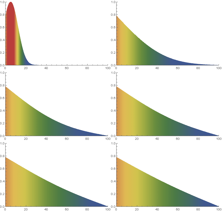
Scale-space theory is a framework for multi-scale signal representation developed by the computer vision, image processing and signal processing communities with complementary motivations from physics and biological vision. It is a formal theory for handling image structures at different scales, by representing an image as a one-parameter family of smoothed images, the scale-space representation, parametrized by the size of the smoothing kernel used for suppressing fine-scale structures. The parameter t in this family is referred to as the ''scale parameter'', with the interpretation that image structures of spatial size smaller than about \sqrt have largely been smoothed away in the scale-space level at scale t. The main type of scale space is the ''linear (Gaussian) scale space'', which has wide applicability as well as the attractive property of being possible to derive from a small set of ''scale-space axioms''. The corresponding scale-space framework encompasses a theory ... [...More Info...] [...Related Items...] OR: [Wikipedia] [Google] [Baidu] |
Scale-space Axioms
In image processing and computer vision, a scale space framework can be used to represent an image as a family of gradually smoothed images. This framework is very general and a variety of scale space representations exist. A typical approach for choosing a particular type of scale space representation is to establish a set of scale-space axioms, describing basic properties of the desired scale-space representation and often chosen so as to make the representation useful in practical applications. Once established, the axioms narrow the possible scale-space representations to a smaller class, typically with only a few free parameters. A set of standard scale space axioms, discussed below, leads to the linear Gaussian scale-space, which is the most common type of scale space used in image processing and computer vision. Scale space axioms for the linear scale-space representation The linear scale space representation L(x, y, t) = (T_t f)(x, y) = g(x, y, t)*f(x, y) of signal f ... [...More Info...] [...Related Items...] OR: [Wikipedia] [Google] [Baidu] |
Anisotropic Diffusion
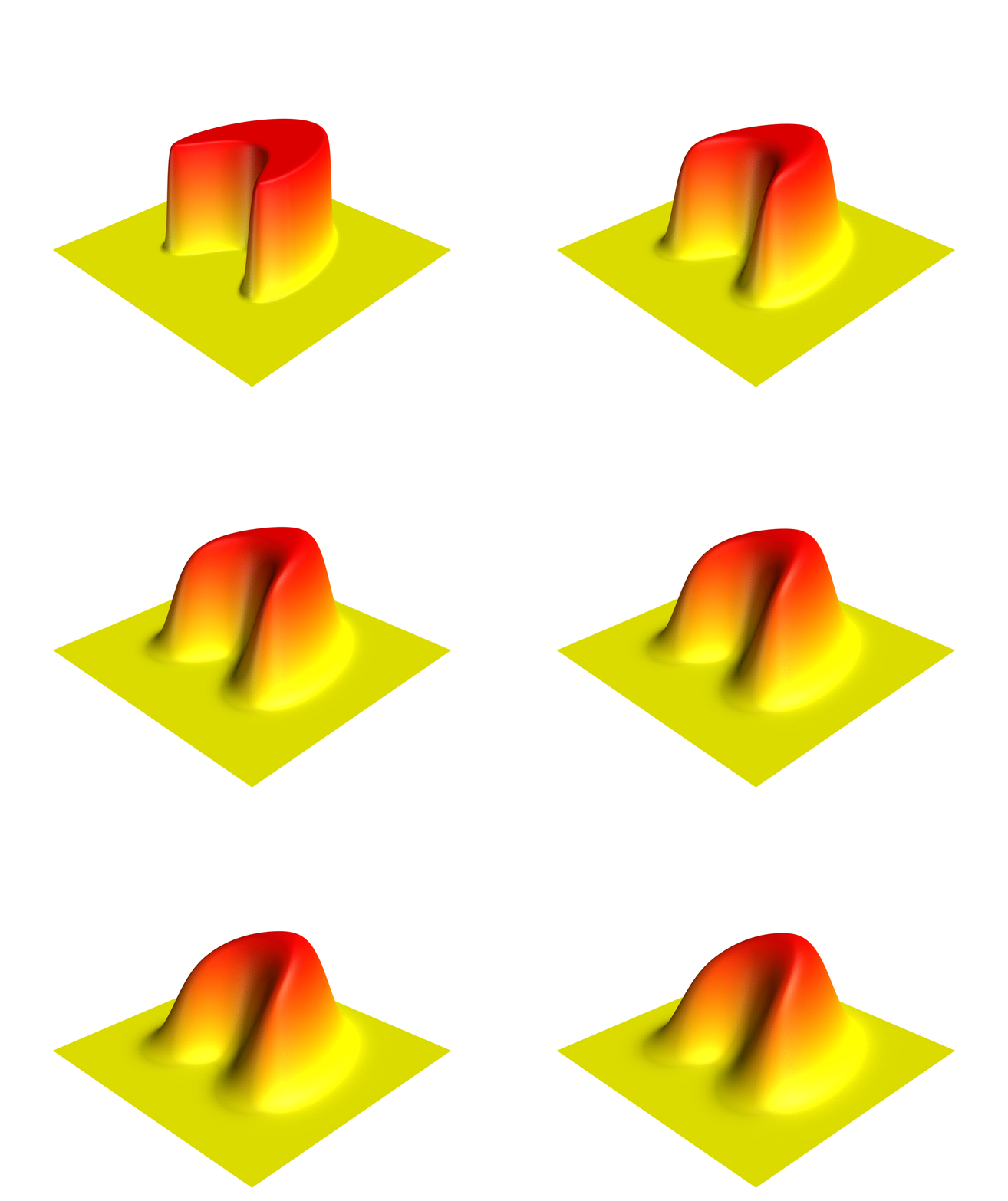
In image processing and computer vision, anisotropic diffusion, also called Perona–Malik diffusion, is a technique aiming at reducing image noise without removing significant parts of the image content, typically edges, lines or other details that are important for the interpretation of the image. Anisotropic diffusion resembles the process that creates a scale space, where an image generates a parameterized family of successively more and more blurred images based on a diffusion process. Each of the resulting images in this family are given as a convolution between the image and a 2D isotropic Gaussian filter, where the width of the filter increases with the parameter. This diffusion process is a ''linear'' and ''space-invariant'' transformation of the original image. Anisotropic diffusion is a generalization of this diffusion process: it produces a family of parameterized images, but each resulting image is a combination between the original image and a filter that depends o ... [...More Info...] [...Related Items...] OR: [Wikipedia] [Google] [Baidu] |
Computer Vision
Computer vision tasks include methods for image sensor, acquiring, Image processing, processing, Image analysis, analyzing, and understanding digital images, and extraction of high-dimensional data from the real world in order to produce numerical or symbolic information, e.g. in the form of decisions. "Understanding" in this context signifies the transformation of visual images (the input to the retina) into descriptions of the world that make sense to thought processes and can elicit appropriate action. This image understanding can be seen as the disentangling of symbolic information from image data using models constructed with the aid of geometry, physics, statistics, and learning theory. The scientific discipline of computer vision is concerned with the theory behind artificial systems that extract information from images. Image data can take many forms, such as video sequences, views from multiple cameras, multi-dimensional data from a 3D scanning, 3D scanner, 3D point clouds ... [...More Info...] [...Related Items...] OR: [Wikipedia] [Google] [Baidu] |
Heat Equation
In mathematics and physics (more specifically thermodynamics), the heat equation is a parabolic partial differential equation. The theory of the heat equation was first developed by Joseph Fourier in 1822 for the purpose of modeling how a quantity such as heat diffuses through a given region. Since then, the heat equation and its variants have been found to be fundamental in many parts of both pure and applied mathematics. Definition Given an open subset of and a subinterval of , one says that a function is a solution of the heat equation if : \frac = \frac + \cdots + \frac, where denotes a general point of the domain. It is typical to refer to as time and as spatial variables, even in abstract contexts where these phrases fail to have their intuitive meaning. The collection of spatial variables is often referred to simply as . For any given value of , the right-hand side of the equation is the Laplace operator, Laplacian of the function . As such, the heat equation is ... [...More Info...] [...Related Items...] OR: [Wikipedia] [Google] [Baidu] |
Multiscale Mathematics
Multiscale modeling or multiscale mathematics is the Branches of science, field of solving problems that have important features at multiple scales of time and/or space. Important problems include multiscale modeling of fluids, solids, polymers, proteins, nucleic acids as well as various physical and chemical phenomena (like adsorption, chemical reactions, diffusion). An example of such problems involve the Navier–Stokes equations for incompressible fluid flow. \begin \rho_0(\partial_t\mathbf+(\mathbf\cdot\nabla)\mathbf)=\nabla\cdot\tau, \\ \nabla\cdot\mathbf=0. \end In a wide variety of applications, the stress tensor \tau is given as a linear function of the gradient \nabla u. Such a choice for \tau has been proven to be sufficient for describing the dynamics of a broad range of fluids. However, its use for more complex fluids such as polymers is dubious. In such a case, it may be necessary to use multiscale modeling to accurately model the system such that the stress tens ... [...More Info...] [...Related Items...] OR: [Wikipedia] [Google] [Baidu] |
Linearity
In mathematics, the term ''linear'' is used in two distinct senses for two different properties: * linearity of a '' function'' (or '' mapping''); * linearity of a '' polynomial''. An example of a linear function is the function defined by f(x)=(ax,bx) that maps the real line to a line in the Euclidean plane R2 that passes through the origin. An example of a linear polynomial in the variables X, Y and Z is aX+bY+cZ+d. Linearity of a mapping is closely related to '' proportionality''. Examples in physics include the linear relationship of voltage and current in an electrical conductor ( Ohm's law), and the relationship of mass and weight. By contrast, more complicated relationships, such as between velocity and kinetic energy, are '' nonlinear''. Generalized for functions in more than one dimension, linearity means the property of a function of being compatible with addition and scaling, also known as the superposition principle. Linearity of a polynomial means that it ... [...More Info...] [...Related Items...] OR: [Wikipedia] [Google] [Baidu] |
Partial Differential Equation
In mathematics, a partial differential equation (PDE) is an equation which involves a multivariable function and one or more of its partial derivatives. The function is often thought of as an "unknown" that solves the equation, similar to how is thought of as an unknown number solving, e.g., an algebraic equation like . However, it is usually impossible to write down explicit formulae for solutions of partial differential equations. There is correspondingly a vast amount of modern mathematical and scientific research on methods to numerically approximate solutions of certain partial differential equations using computers. Partial differential equations also occupy a large sector of pure mathematical research, in which the usual questions are, broadly speaking, on the identification of general qualitative features of solutions of various partial differential equations, such as existence, uniqueness, regularity and stability. Among the many open questions are the existence ... [...More Info...] [...Related Items...] OR: [Wikipedia] [Google] [Baidu] |
Partial Derivative
In mathematics, a partial derivative of a function of several variables is its derivative with respect to one of those variables, with the others held constant (as opposed to the total derivative, in which all variables are allowed to vary). Partial derivatives are used in vector calculus and differential geometry. The partial derivative of a function f(x, y, \dots) with respect to the variable x is variously denoted by It can be thought of as the rate of change of the function in the x-direction. Sometimes, for the partial derivative of z with respect to x is denoted as \tfrac. Since a partial derivative generally has the same arguments as the original function, its functional dependence is sometimes explicitly signified by the notation, such as in: f'_x(x, y, \ldots), \frac (x, y, \ldots). The symbol used to denote partial derivatives is ∂. One of the first known uses of this symbol in mathematics is by Marquis de Condorcet from 1770, who used it for partial differ ... [...More Info...] [...Related Items...] OR: [Wikipedia] [Google] [Baidu] |
Diffusion
Diffusion is the net movement of anything (for example, atoms, ions, molecules, energy) generally from a region of higher concentration to a region of lower concentration. Diffusion is driven by a gradient in Gibbs free energy or chemical potential. It is possible to diffuse "uphill" from a region of lower concentration to a region of higher concentration, as in spinodal decomposition. Diffusion is a stochastic process due to the inherent randomness of the diffusing entity and can be used to model many real-life stochastic scenarios. Therefore, diffusion and the corresponding mathematical models are used in several fields beyond physics, such as statistics, probability theory, information theory, neural networks, finance, and marketing. The concept of diffusion is widely used in many fields, including physics (Molecular diffusion, particle diffusion), chemistry, biology, sociology, economics, statistics, data science, and finance (diffusion of people, ideas, data and price v ... [...More Info...] [...Related Items...] OR: [Wikipedia] [Google] [Baidu] |
Diffusion Equation
The diffusion equation is a parabolic partial differential equation. In physics, it describes the macroscopic behavior of many micro-particles in Brownian motion, resulting from the random movements and collisions of the particles (see Fick's laws of diffusion). In mathematics, it is related to Markov processes, such as random walks, and applied in many other fields, such as materials science, information theory, and biophysics. The diffusion equation is a special case of the convection–diffusion equation when bulk velocity is zero. It is equivalent to the heat equation under some circumstances. Statement The equation is usually written as: \frac = \nabla \cdot \big D(\phi,\mathbf) \ \nabla\phi(\mathbf,t) \big where is the density of the diffusing material at location and time and is the collective diffusion coefficient for density at location ; and represents the vector differential operator del. If the diffusion coefficient depends on the density then the equatio ... [...More Info...] [...Related Items...] OR: [Wikipedia] [Google] [Baidu] |
Rotational Invariance
In mathematics, a function defined on an inner product space is said to have rotational invariance if its value does not change when arbitrary rotations are applied to its argument. Mathematics Functions For example, the function : f(x,y) = x^2 + y^2 is invariant under rotations of the plane around the origin, because for a rotated set of coordinates through any angle ''θ'' : x' = x \cos \theta - y \sin \theta : y' = x \sin \theta + y \cos \theta the function, after some cancellation of terms, takes exactly the same form : f(x',y') = ^2 + ^2 The rotation of coordinates can be expressed using matrix form using the rotation matrix, : \begin x' \\ y' \\ \end = \begin \cos \theta & -\sin \theta \\ \sin \theta & \cos \theta \\ \end\begin x \\ y \\ \end , or symbolically, = Rx. Symbolically, the rotation invariance of a real-valued function of two real variables is : f(\mathbf') = f(\mathbf) = f(\mathbf) In words, the function of the rotated coordinates takes exactly the ... [...More Info...] [...Related Items...] OR: [Wikipedia] [Google] [Baidu] |


