Kaplan–Meier estimator

The Kaplan–Meier estimator, also known as the product limit estimator, is a non-parametric statistic used to estimate the survival function from lifetime data. In medical research, it is often used to measure the fraction of patients living for a certain amount of time after treatment. In other fields, Kaplan–Meier estimators may be used to measure the length of time people remain unemployed after a job loss, the time-to-failure of machine parts, or how long fleshy fruits remain on plants before they are removed by frugivores. The estimator is named after Edward L. Kaplan and Paul Meier, who each submitted similar manuscripts to the '' Journal of the American Statistical Association''. The journal editor, John Tukey, convinced them to combine their work into one paper, which has been cited almost 61,000 times since its publication in 1958.

The estimator of the survival function $S(t)$ (the probability that life is longer than $t$) is given by:

: $\widehat S(t) = \prod\limits_ \left(1 - \frac\right),$

with $t_i$ a time when at least one event happened, ''d''_''i'' the ''number of events'' (e.g., deaths) that happened at time $t_i$, and $n_i$ the ''individuals known to have survived'' (have not yet had an event or been censored) up to time $t_i$.

Basic concepts

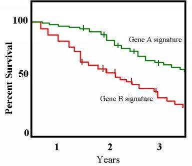
A plot of the Kaplan–Meier estimator is a series of declining horizontal steps which, with a large enough sample size, approaches the true survival function for that population. The value of the survival function between successive distinct sampled observations ("clicks") is assumed to be constant.

An important advantage of the Kaplan–Meier curve is that the method can take into account some types of censored data, particularly ''right-censoring'', which occurs if a patient withdraws from a study, is lost to follow-up, or is alive without event occurrence at last follow-up. On the plot, small vertical tick-marks state individual patients whose survival times have been right-censored. When no truncation or censoring occurs, the Kaplan–Meier curve is the complement of the empirical distribution function.

In medical statistics, a typical application might involve grouping patients into categories, for instance, those with Gene A profile and those with Gene B profile. In the graph, patients with Gene B die much quicker than those with Gene A. After two years, about 80% of the Gene A patients survive, but less than half of patients with Gene B.

To generate a Kaplan–Meier estimator, at least two pieces of data are required for each patient (or each subject): the status at last observation (event occurrence or right-censored), and the time to event (or time to censoring). If the survival functions between two or more groups are to be compared, then a third piece of data is required: the group assignment of each subject.

Problem definition

Let $\tau\ge 0$ be a random variable, which we think of as the time until an event of interest takes place. As indicated above, the goal is to estimate the survival function $S$ underlying $\tau$. Recall that this function is defined as

:$S(t) = \operatorname(\tau > t )$, where $t=0,1,\dots$ is the time.

Let $\tau_1,\dots,\tau_n\ge 0$ be independent, identically distributed random variables, whose common distribution is that of $\tau$: $\tau_j$ is the random time when some event $j$ happened. The data available for estimating $S$ is not $(\tau_j)_$, but the list of pairs $(\, ( \tilde \tau_j, c_j )\, )_$ where for j\in := \, $c_j\ge 0$ is a fixed, deterministic integer, the censoring time of event $j$ and $\tilde \tau_j = \min(\tau_j,c_j)$. In particular, the information available about the timing of event $j$ is whether the event happened before the fixed time $c_j$ and if so, then the actual time of the event is also available. The challenge is to estimate $S(t)$ given this data.

Derivation of the Kaplan–Meier estimator

Here, we show two derivations of the Kaplan–Meier estimator. Both are based on rewriting the survival function in terms of what is sometimes called hazard, or mortality rates. However, before doing this it is worthwhile to consider a naive estimator.

A naive estimator

To understand the power of the Kaplan–Meier estimator, it is worthwhile to first describe a naive estimator of the survival function.

Fix k\in =\ and let $t>0$. A basic argument shows that the following proposition holds:

:Proposition 1: If the censoring time $c_k$ of event $k$ exceeds $t$ ($c_k\ge t$), then $\tilde \tau_k\ge t$ if and only if $\tau_k\ge t$.

Let $k$ be such that $c_k\ge t$. It follows from the above proposition that

: $\operatorname(\tau_k\ge t) = \operatorname(\tilde \tau_k\ge t).$

Let $X_k = \mathbb(\tilde \tau_k\ge t)$ and consider only those $k\in C(t) := \$, i.e. the events for which the outcome was not censored before time $t$. Let $m(t)=, C(t),$ be the number of elements in $C(t)$. Note that the set $C(t)$ is not random and so neither is $m(t)$. Furthermore, $(X_k)_$ is a sequence of independent, identically distributed Bernoulli random variables with common parameter $S(t)=\operatorname(\tau\ge t)$. Assuming that $m(t)>0$, this suggests to estimate $S(t)$ using

: $\hat S_\text(t) = \frac \sum_ X_k = \frac = \frac,$

where the second equality follows because $\tilde \tau_k\ge t$ implies $c_k\ge t$, while the last equality is simply a change of notation.

The quality of this estimate is governed by the size of $m(t)$. This can be problematic when $m(t)$ is small, which happens, by definition, when a lot of the events are censored. A particularly unpleasant property of this estimator, that suggests that perhaps it is not the "best" estimator, is that it ignores all the observations whose censoring time precedes $t$. Intuitively, these observations still contain information about $S(t)$: For example, when for many events with $c_k < t$, \tilde \tau_k also holds, we can infer that events often happen early, which implies that $\operatorname(\tau\le t)$ is large, which, through $S(t) = 1-\operatorname(\tau\le t)$ means that $S(t)$ must be small. However, this information is ignored by this naive estimator. The question is then whether there exists an estimator that makes a better use of all the data. This is what the Kaplan–Meier estimator accomplishes. Note that the naive estimator cannot be improved when censoring does not take place; so whether an improvement is possible critically hinges upon whether censoring is in place.

The plug-in approach

By elementary calculations,

: \begin
S(t) & = \operatorname(\tau > t\mid\tau > t-1)\operatorname(\tau > t-1) \\ pt & = (1-\operatorname(\tau\le t\mid\tau > t-1)) \operatorname(\tau > t-1)\\ pt & = (1-\operatorname(\tau=t\mid\tau \ge t)) \operatorname(\tau > t-1) \\ pt & = q(t) S(t-1)\,,
\end

where the one but last equality used that $\tau$ is integer valued and for the last line we introduced

: $q(t) = 1-\operatorname(\tau=t\mid\tau\ge t).$

By a recursive expansion of the equality $S(t) = q(t) S(t-1)$, we get

: $S(t) = q(t) q(t-1) \cdots q(0).$

Note that here $q(0) = 1-\operatorname(\tau=0\mid\tau > -1) = 1-\operatorname(\tau=0)$.

The Kaplan–Meier estimator can be seen as a "plug-in estimator" where each $q(s)$ is estimated based on the data and the estimator of $S(t)$ is obtained as a product of these estimates.

It remains to specify how $q(s)=1-\operatorname(\tau=s\mid\tau\ge s)$ is to be estimated. By Proposition 1, for any k\in /math> such that $c_k\ge s$, $\operatorname(\tau=s) = \operatorname(\tilde \tau_k=s)$ and $\operatorname(\tau\ge s) = \operatorname(\tilde \tau_k\ge s)$ both hold. Hence, for any
k\in such that $c_k\ge s$,

: $\operatorname(\tau=s, \tau\ge s) = \operatorname(\tilde \tau_k=s)/\operatorname(\tilde \tau_k\ge s).$

By a similar reasoning that lead to the construction of the naive estimator above, we arrive at the estimator

: $\hat q(s) = 1 - \frac = 1 - \frac$

(think of estimating the numerator and denominator separately in the definition of the "hazard rate" $\operatorname(\tau=s, \tau\ge s)$). The Kaplan–Meier estimator is then given by

: $\hat S(t) = \prod_^t \hat q(s).$

The form of the estimator stated at the beginning of the article can be obtained by some further algebra. For this, write $\hat q(s)=1-d(s)/n(s)$ where, using the actuarial science terminology, $d(s)=, \,$ is the number of known deaths at time $s$, while $n(s)=, \,$ is the number of those persons who are alive (and not being censored) at time $s-1$.

Note that if $d(s)=0$, $\hat q(s)=1$. This implies that we can leave out from the product defining $\hat S(t)$ all those terms where $d(s)=0$. Then, letting 0\le t_1 be the times $s$ when $d(s)>0$, $d_i = d(t_i)$ and $n_i = n(t_i)$, we arrive at the form of the Kaplan–Meier estimator given at the beginning of the article:

: $\hat S(t) = \prod_ \left(1-\frac\right).$

As opposed to the naive estimator, this estimator can be seen to use the available information more effectively: In the special case mentioned beforehand, when there are many early events recorded, the estimator will multiply many terms with a value below one and will thus take into account that the survival probability cannot be large.

Derivation as a maximum likelihood estimator

Kaplan–Meier estimator can be derived from maximum likelihood estimation of hazard function. More specifically given $d_i$ as the number of events and $n_i$ the total individuals at risk at time $t_i$, discrete hazard rate $h_i$ can be defined as the probability of an individual with an event at time $t_i$. Then survival rate can be defined as:

: $S(t) = \prod\limits_ (1-h_i)$

and the likelihood function for the hazard function up to time $t_i$ is:

: $\mathcal(h_\mid d_,n_) = \prod_^i h_j^(1-h_j)^$

therefore the log likelihood will be:

: $\log(\mathcal) = \sum_^i \left(d_j\log(h_j)+(n_j-d_j)\log(1-h_j)\right)$

finding the maximum of log likelihood with respect to $h_i$ yields:

: $\frac = \frac-\frac = 0 \Rightarrow \widehat_i=\frac$

where hat is used to denote maximum likelihood estimation. Given this result, we can write:

: $\widehat S(t) = \prod\limits_ \left(1 - \widehat_i\right) = \prod\limits_ \left(1 - \frac\right)$

Benefits and limitations

The Kaplan–Meier estimator is one of the most frequently used methods of survival analysis. The estimate may be useful to examine recovery rates, the probability of death, and the effectiveness of treatment. It is limited in its ability to estimate survival adjusted for covariates; parametric survival models and the Cox proportional hazards model may be useful to estimate covariate-adjusted survival.

Statistical considerations

The Kaplan–Meier estimator is a statistic, and several estimators are used to approximate its variance. One of the most common estimators is Greenwood's formula:

:$\widehat \left( \widehat S(t) \right) = \widehat S(t)^2 \sum_ \frac,$

where $d_i$ is the number of cases and $n_i$ is the total number of observations, for $t_i < t$.

In some cases, one may wish to compare different Kaplan–Meier curves. This can be done by the log rank test, and the Cox proportional hazards test.

Other statistics that may be of use with this estimator are pointwise confidence intervals, the Hall-Wellner band and the equal-precision band.

Software

* Mathematica: the built-in function SurvivalModelFit creates survival models.
* SAS: The Kaplan–Meier estimator is implemented in the proc lifetest procedure.
* R: the Kaplan–Meier estimator is available as part of the survival package.
* Stata: the command sts returns the Kaplan–Meier estimator.
* Python: the lifelines package includes the Kaplan–Meier estimator.
* MATLAB: the ecdf function with the 'function','survivor' arguments can calculate or plot the Kaplan–Meier estimator.
* StatsDirect: The Kaplan–Meier estimator is implemented in the Survival Analysis menu.
* SPSS: The Kaplan–Meier estimator is implemented in the Analyze > Survival > Kaplan-Meier... menu.
* Julia: the Survival.jl package includes the Kaplan–Meier estimator.

See also

* Survival Analysis
* Frequency of exceedance
* Median lethal dose
* Nelson–Aalen estimator

References

Further reading

*
*
*
*

External links

*
*
*

{{DEFAULTSORT:Kaplan-Meier estimator
Estimator
Actuarial science
Survival analysis
Reliability engineering