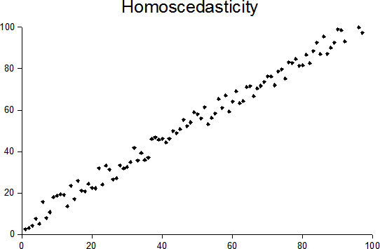
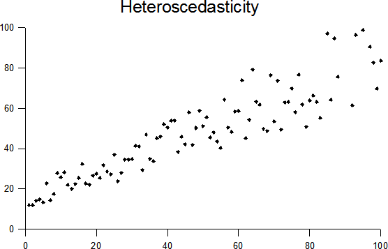
Heteroscedasticity

In statistics, a sequence (or a vector) of random variables is homoscedastic () if all its random variables have the same finite variance. This is also known as homogeneity of variance. The complementary notion is called heteroscedasticity. The spellings ''homoskedasticity'' and ''heteroskedasticity'' are also frequently used.

Assuming a variable is homoscedastic when in reality it is heteroscedastic () results in unbiased but inefficient point estimates and in biased estimates of standard errors, and may result in overestimating the goodness of fit as measured by the Pearson coefficient.

The existence of heteroscedasticity is a major concern in regression analysis and the analysis of variance, as it invalidates statistical tests of significance that assume that the modelling errors all have the same variance. While the ordinary least squares estimator is still unbiased in the presence of heteroscedasticity, it is inefficient and generalized least squares should be used instead.

Because heteroscedasticity concerns expectations of the second moment of the errors, its presence is referred to as misspecification of the second order.

The econometrician Robert Engle was awarded the 2003 Nobel Memorial Prize for Economics for his studies on regression analysis in the presence of heteroscedasticity, which led to his formulation of the autoregressive conditional heteroscedasticity (ARCH) modeling technique.

Definition

Consider the linear regression equation $y_i= x_i \beta_i + \varepsilon_i,\ i = 1,\ldots, N,$ where the dependent random variable $y_i$ equals the deterministic variable $x_i$ times coefficient $\beta$ plus a random disturbance term $\varepsilon_i$ that has mean zero. The disturbances are homoscedastic if the variance of $\varepsilon_i$ is a constant $\sigma^2$; otherwise, they are heteroscedastic. In particular, the disturbances are heteroscedastic if the variance of $\varepsilon_i$ depends on $i$ or on the value of $x_i$. One way they might be heteroscedastic is if $\sigma_i^2= x_i \sigma^2$ (an example of a scedastic function), so the variance is proportional to the value of $x$.

More generally, if the variance-covariance matrix of disturbance $\varepsilon_i$ across $i$ has a nonconstant diagonal, the disturbance is heteroscedastic. The matrices below are covariances when there are just three observations across time. The disturbance in matrix A is homoscedastic; this is the simple case where OLS is the best linear unbiased estimator. The disturbances in matrices B and C are heteroscedastic. In matrix B, the variance is time-varying, increasing steadily across time; in matrix C, the variance depends on the value of $x$. The disturbance in matrix D is homoscedastic because the diagonal variances are constant, even though the off-diagonal covariances are non-zero and ordinary least squares is inefficient for a different reason: serial correlation.
:$\begin A &= \sigma^2\begin 1 & 0 & 0 \\ 0 & 1 & 0 \\ 0 & 0 & 1 \\ \end & B &= \sigma^2\begin 1 & 0 & 0 \\ 0 & 2 & 0 \\ 0 & 0 & 3 \\ \end & C &= \sigma^2\begin x_1 & 0 & 0 \\ 0 & x_2 & 0 \\ 0 & 0 & x_3 \\ \end & D &= \sigma^2\begin 1 & \rho & \rho^2 \\ \rho & 1 & \rho \\ \rho^2 & \rho & 1 \\ \end \end$

Examples

Heteroscedasticity often occurs when there is a large difference among the sizes of the observations.

* A classic example of heteroscedasticity is that of income versus expenditure on meals. As one's income increases, the variability of food consumption will increase. A poorer person will spend a rather constant amount by always eating inexpensive food; a wealthier person may occasionally buy inexpensive food and at other times eat expensive meals. Those with higher incomes display a greater variability of food consumption.
* Imagine you are watching a rocket take off nearby and measuring the distance it has travelled once each second. In the first couple of seconds your measurements may be accurate to the nearest centimeter, say. However, 5 minutes later as the rocket recedes into space, the accuracy of your measurements may only be good to 100 m, because of the increased distance, atmospheric distortion and a variety of other factors. The data you collect would exhibit heteroscedasticity.

Consequences of heteroscedasticity

One of the assumptions of the classical linear regression model is that there is no heteroscedasticity. Breaking this assumption means that the Gauss–Markov theorem does not apply, meaning that OLS estimators are not the Best Linear Unbiased Estimators (BLUE) and their variance is not the lowest of all other unbiased estimators.
Heteroscedasticity does ''not'' cause ordinary least squares coefficient estimates to be biased, although it can cause ordinary least squares estimates of the variance (and, thus, standard errors) of the coefficients to be biased, possibly above or below the true of population variance. Thus, regression analysis using heteroscedastic data will still provide an unbiased estimate for the relationship between the predictor variable and the outcome, but standard errors and therefore inferences obtained from data analysis are suspect. Biased standard errors lead to biased inference, so results of hypothesis tests are possibly wrong. For example, if OLS is performed on a heteroscedastic data set, yielding biased standard error estimation, a researcher might fail to reject a null hypothesis at a given significance level, when that null hypothesis was actually uncharacteristic of the actual population (making a type II error).

Under certain assumptions, the OLS estimator has a normal asymptotic distribution when properly normalized and centered (even when the data does not come from a normal distribution). This result is used to justify using a normal distribution, or a chi square distribution (depending on how the test statistic is calculated), when conducting a hypothesis test. This holds even under heteroscedasticity. More precisely, the OLS estimator in the presence of heteroscedasticity is asymptotically normal, when properly normalized and centered, with a variance-covariance matrix that differs from the case of homoscedasticity. In 1980, White proposed a consistent estimator for the variance-covariance matrix of the asymptotic distribution of the OLS estimator. This validates the use of hypothesis testing using OLS estimators and White's variance-covariance estimator under heteroscedasticity.

Heteroscedasticity is also a major practical issue encountered in ANOVA problems.
The F test can still be used in some circumstances.

However, it has been said that students in econometrics should not overreact to heteroscedasticity. One author wrote, "unequal error variance is worth correcting only when the problem is severe." In addition, another word of caution was in the form, "heteroscedasticity has never been a reason to throw out an otherwise good model." With the advent of heteroscedasticity-consistent standard errors allowing for inference without specifying the conditional second moment of error term, testing conditional homoscedasticity is not as important as in the past.

For any non-linear model (for instance Logit and Probit models), however, heteroscedasticity has more severe consequences: the maximum likelihood estimates (MLE) of the parameters will be biased, as well as inconsistent (unless the likelihood function is modified to correctly take into account the precise form of heteroscedasticity). Yet, in the context of binary choice models (Logit or Probit), heteroscedasticity will only result in a positive scaling effect on the asymptotic mean of the misspecified MLE (i.e. the model that ignores heteroscedasticity). As a result, the predictions which are based on the misspecified MLE will remain correct. In addition, the misspecified Probit and Logit MLE will be asymptotically normally distributed which allows performing the usual significance tests (with the appropriate variance-covariance matrix). However, regarding the general hypothesis testing, as pointed out by Greene, “simply computing a robust covariance matrix for an otherwise inconsistent estimator does not give it redemption. Consequently, the virtue of a robust covariance matrix in this setting is unclear.”

Correcting for heteroscedasticity

There are five common corrections for heteroscedasticity. They are:
* View logarithmized data. Non-logarithmized series that are growing exponentially often appear to have increasing variability as the series rises over time. The variability in percentage terms may, however, be rather stable.
* Use a different specification for the model (different ''X'' variables, or perhaps non-linear transformations of the ''X'' variables).
* Apply a weighted least squares estimation method, in which OLS is applied to transformed or weighted values of ''X'' and ''Y''. The weights vary over observations, usually depending on the changing error variances. In one variation the weights are directly related to the magnitude of the dependent variable, and this corresponds to least squares percentage regression.
* Heteroscedasticity-consistent standard errors (HCSE), while still biased, improve upon OLS estimates. HCSE is a consistent estimator of standard errors in regression models with heteroscedasticity. This method corrects for heteroscedasticity without altering the values of the coefficients. This method may be superior to regular OLS because if heteroscedasticity is present it corrects for it, however, if the data is homoscedastic, the standard errors are equivalent to conventional standard errors estimated by OLS. Several modifications of the White method of computing heteroscedasticity-consistent standard errors have been proposed as corrections with superior finite sample properties.
* Use MINQUE or even the customary estimators $s_i^2 = (n_i - 1)^ \sum_j \left(y_ - \bar_i\right)^2$ (for $i=1,2,...,k$ independent samples with $j=1, 2, ..., n_i$ observations each), whose efficiency losses are not substantial when the number of observations per sample is large ($n_i > 5$), especially for small number of independent samples.

Testing for heteroscedasticity

Residuals can be tested for homoscedasticity using the Breusch–Pagan test, which performs an auxiliary regression of the squared residuals on the independent variables. From this auxiliary regression, the explained sum of squares is retained, divided by two, and then becomes the test statistic for a chi-squared distribution with the degrees of freedom equal to the number of independent variables. The null hypothesis of this chi-squared test is homoscedasticity, and the alternative hypothesis would indicate heteroscedasticity. Since the Breusch–Pagan test is sensitive to departures from normality or small sample sizes, the Koenker–Bassett or 'generalized Breusch–Pagan' test is commonly used instead. From the auxiliary regression, it retains the R-squared value which is then multiplied by the sample size, and then becomes the test statistic for a chi-squared distribution (and uses the same degrees of freedom). Although it is not necessary for the Koenker–Bassett test, the Breusch–Pagan test requires that the squared residuals also be divided by the residual sum of squares divided by the sample size. Testing for groupwise heteroscedasticity can be done with the Goldfeld–Quandt test.

List of heteroscedasticity tests

Although tests for heteroscedasticity between groups can formally be considered as a special case of testing within regression models, some tests have structures specific to this case.

Tests in regression

*Levene's test
* Goldfeld–Quandt test
* Park test
* Glejser test
* Brown–Forsythe test
* Harrison–McCabe test
*Breusch–Pagan test
* White test
* Cook–Weisberg test

Tests for grouped data

*F-test of equality of variances
* Cochran's C test
* Hartley's test
* Bartlett's test

Generalisations

Homoscedastic distributions

Two or more normal distributions, $N(\mu_1,\Sigma_1), N(\mu_2,\Sigma_2),$ are both homoscedastic and lack Serial correlation if they share the same diagonals in their covariance matrix, $\Sigma_1 = \Sigma_2,\ \forall i=j.$ and their non-diagonal entries are zero. Homoscedastic distributions are especially useful to derive statistical pattern recognition and machine learning algorithms. One popular example of an algorithm that assumes homoscedasticity is Fisher's linear discriminant analysis.
The concept of homoscedasticity can be applied to distributions on spheres.

Multivariate data

The study of homescedasticity and heteroscedasticity has been generalized to the multivariate case, which deals with the covariances of vector observations instead of the variance of scalar observations. One version of this is to use covariance matrices as the multivariate measure of dispersion. Several authors have considered tests in this context, for both regression and grouped-data situations. Bartlett's test for heteroscedasticity between grouped data, used most commonly in the univariate case, has also been extended for the multivariate case, but a tractable solution only exists for 2 groups. Approximations exist for more than two groups, and they are both called Box's M test.

See also

* Heterogeneity
* Spherical error

References

Further reading

Most statistics textbooks will include at least some material on homoscedasticity and heteroscedasticity. Some examples are:
*
*
*
*
*
*

External links

* by Mark Thoma

{{statistics

Statistical deviation and dispersion
Regression analysis

ja:ARCHモデル#分散不均一性