Ratio distribution

A ratio distribution (also known as a quotient distribution) is a probability distribution constructed as the distribution of the ratio of random variables having two other known distributions.
Given two (usually independent) random variables ''X'' and ''Y'', the distribution of the random variable ''Z'' that is formed as the ratio ''Z'' = ''X''/''Y'' is a ''ratio distribution''.

An example is the Cauchy distribution (also called the ''normal ratio distribution''), which comes about as the ratio of two normally distributed variables with zero mean.
Two other distributions often used in test-statistics are also ratio distributions:
the ''t''-distribution arises from a Gaussian random variable divided by an independent chi-distributed random variable,
while the ''F''-distribution originates from the ratio of two independent chi-squared distributed random variables.
More general ratio distributions have been considered in the literature.

Often the ratio distributions are heavy-tailed, and it may be difficult to work with such distributions and develop an associated statistical test.
A method based on the median has been suggested as a "work-around".

Algebra of random variables

The ratio is one type of algebra for random variables:
Related to the ratio distribution are the product distribution, sum distribution and difference distribution. More generally, one may talk of combinations of sums, differences, products and ratios.
Many of these distributions are described in Melvin D. Springer's book from 1979 ''The Algebra of Random Variables''.

The algebraic rules known with ordinary numbers do not apply for the algebra of random variables.
For example, if a product is ''C = AB'' and a ratio is ''D=C/A'' it does not necessarily mean that the distributions of ''D'' and ''B'' are the same.
Indeed, a peculiar effect is seen for the Cauchy distribution: The product and the ratio of two independent Cauchy distributions (with the same scale parameter and the location parameter set to zero) will give the same distribution.
This becomes evident when regarding the Cauchy distribution as itself a ratio distribution of two Gaussian distributions of zero means: Consider two Cauchy random variables, $C_1$ and $C_2$ each constructed from two Gaussian distributions $C_1=G_1/G_2$ and $C_2 = G_3/G_4$ then

: $\frac = \frac = \frac = \frac \times \frac = C_1 \times C_3,$

where $C_3 = G_4/G_3$. The first term is the ratio of two Cauchy distributions while the last term is the product of two such distributions.

Derivation

A way of deriving the ratio distribution of $Z = X/Y$ from the joint distribution of the two other random variables ''X , Y'' , with joint pdf $p_(x,y)$, is by integration of the following form

: $p_Z(z) = \int^_ , y, \, p_(zy, y) \, dy.$

If the two variables are independent then $p_(x,y) = p_X(x) p_Y(y)$ and this becomes

: $p_Z(z) = \int^_ , y, \, p_X(zy) p_Y(y) \, dy.$

This may not be straightforward. By way of example take the classical problem of the ratio of two standard Gaussian samples. The joint pdf is

:$p_(x,y) = \frac \exp\left(-\frac \right) \exp \left(-\frac \right)$

Defining $Z = X/Y$ we have

:$\begin p_Z(z) &= \frac \int_^ \, , y, \, \exp\left(-\frac \right) \, \exp\left(-\frac \right) \, dy \\ &= \frac \int_^ \,, y, \, \exp\left(-\frac \right) \, dy \end$
Using the known definite integral $\int_0^ \, x \, \exp\left(-cx^2 \right) \, dx = \frac$ we get

:$p_Z(z) = \frac$
which is the Cauchy distribution, or Student's ''t'' distribution with ''n'' = 1

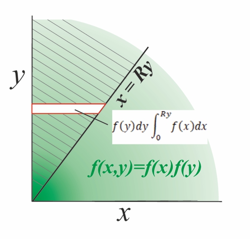
The Mellin transform has also been suggested for derivation of ratio distributions.

In the case of positive independent variables, proceed as follows. The diagram shows a separable bivariate distribution $f_(x,y)=f_x(x)f_y(y)$ which has support in the positive quadrant $x,y > 0$ and we wish to find the pdf of the ratio $R= X/Y$. The hatched volume above the line $y = x/ R$ represents the cumulative distribution of the function $f_(x,y)$ multiplied with the logical function $X/Y \le R$. The density is first integrated in horizontal strips; the horizontal strip at height ''y'' extends from ''x'' = 0 to ''x = Ry'' and has incremental probability $f_y(y)dy \int_0^ f_x(x) \,dx$.

Secondly, integrating the horizontal strips upward over all ''y'' yields the volume of probability above the line
:$F_R(R) = \int_0^\infty f_y(y) \left(\int_0^ f_x(x)dx \right) dy$
Finally, differentiate $F_R(R)$ with respect to $R$ to get the pdf $f_R(R)$.
: f_R(R) = \frac \left \int_0^\infty f_y(y) \left(\int_0^ f_x(x)dx \right) dy \right
Move the differentiation inside the integral:
:$f_R(R) = \int_0^\infty f_y(y) \left(\frac \int_0^ f_x(x)dx \right) dy$
and since
:$\frac \int_0^ f_x(x)dx = yf_x(Ry)$
then
:$f_R(R) = \int_0^\infty f_y(y) \; f_x(Ry) \; y \; dy$
As an example, find the pdf of the ratio ''R'' when
: $f_x(x) = \alpha e^, \;\;\;\; f_y(y) = \beta e^, \;\;\; x,y \ge 0$

We have
:$\int_0^ f_x(x)dx = - e^ \vert_0^ = 1- e^$
thus
:$\begin F_R(R) &= \int_0^\infty f_y(y) \left( 1- e^ \right) dy =\int_0^\infty \beta e^ \left( 1- e^ \right) dy \\ & = 1 - \frac \\ & = \frac \end$
Differentiation wrt. ''R'' yields the pdf of ''R''
:$f_R(R) =\frac \left( \frac \right) = \frac$

Moments of random ratios

From Mellin transform theory, for distributions existing only on the positive half-line $x \ge 0$, we have the product identity \operatorname UV)^p = \operatorname ^p \;\; \operatorname ^p provided $U, \; V$ are independent. For the case of a ratio of samples like \operatorname X/Y)^p, in order to make use of this identity it is necessary to use moments of the inverse distribution. Set $1/Y = Z$ such that \operatorname XZ)^p = \operatorname ^p \; \operatorname ^ /math>.
Thus, if the moments of $X^p$ and $Y^$ can be determined separately, then the moments of $X/Y$ can be found. The moments of $Y^$ are determined from the inverse pdf of $Y$ , often a tractable exercise. At simplest, \operatorname Y^ =\int_0^\infty y^ f_y(y)\,dy .

To illustrate, let $X$ be sampled from a standard Gamma distribution
: $x^e^/\Gamma(\alpha)$ whose $p$-th moment is $\Gamma(\alpha + p) / \Gamma(\alpha)$.

$Z = Y^$is sampled from an inverse Gamma distribution with parameter $\beta$ and has pdf $\; \Gamma^(\beta) z^ e^$. The moments of this pdf are
: \operatorname ^p \operatorname ^= \frac , \; p<\beta.

Multiplying the corresponding moments gives
: \operatorname X/Y)^p\operatorname ^p\; \operatorname ^= \frac \frac , \; p<\beta.

Independently, it is known that the ratio of the two Gamma samples $R = X/Y$ follows the Beta Prime distribution:
:$f_(r, \alpha, \beta) = B(\alpha, \beta)^ r^ (1+r)^$ whose moments are \operatorname ^p \frac

Substituting $\Beta(\alpha, \beta) =\frac$ we have
\operatorname ^p= \frac \Bigg/
\frac =
\frac
which is consistent with the product of moments above.

Means and variances of random ratios

In the Product distribution section, and derived from Mellin transform theory (see section above), it is found that the mean of a product of independent variables is equal to the product of their means. In the case of ratios, we have

:$\operatorname(X/Y) = \operatorname(X)\operatorname(1/Y)$

which, in terms of probability distributions, is equivalent to

: $\operatorname(X/Y) = \int_^\infty x f_x(x) \, dx \times \int_^\infty y^ f_y(y) \, dy$

Note that $\operatorname(1/Y) \neq \frac$ i.e., $\int_^\infty y^ f_y(y) \, dy \ne \frac$

The variance of a ratio of independent variables is

: \begin \operatorname(X/Y) & = \operatorname( /Y2) - \operatorname(X/Y)
\\ & = \operatorname(X^2) \operatorname(1/Y^2) -
\operatorname^2(X) \operatorname^2(1/Y)
\end

Normal ratio distributions

Uncorrelated central normal ratio

When ''X'' and ''Y'' are independent and have a Gaussian distribution with zero mean, the form of their ratio distribution is a Cauchy distribution.
This can be derived by setting $Z = X/Y = \tan \theta$ then showing that $\theta$ has circular symmetry. For a bivariate uncorrelated Gaussian distribution we have
: $\begin p(x,y) &= \tfrac e^ \times \tfrac e^ \\ &= \tfrac e^ \\ & = \tfrac e^ \text r^2 = x^2 + y^2 \end$

If $p(x,y)$ is a function only of ''r'' then $\theta$ is uniformly distributed on , 2\pi with density $1/2\pi$ so the problem reduces to finding the probability distribution of ''Z'' under the mapping
: $Z = X/Y = \tan \theta$
We have, by conservation of probability
: $p_z(z) , dz, = p_(\theta), d\theta,$
and since $dz/d\theta = 1/ \cos^2 \theta$
: $p_z(z) = \frac = \tfrac$
and setting $\cos^2 \theta = \frac= \frac$ we get
: $p_z(z) = \frac$
There is a spurious factor of 2 here. Actually, two values of $\theta$ spaced by $\pi$ map onto the same value of ''z'', the density is doubled, and the final result is
: $p_z(z) = \frac , \;\; -\infty < z < \infty$

When either of the two Normal distributions is non-central then the result for the distribution of the ratio is much more complicated and is given below in the succinct form presented by David Hinkley. The trigonometric method for a ratio does however extend to radial distributions like bivariate normals or a bivariate Student ''t'' in which the density depends only on radius $r = \sqrt$. It does not extend to the ratio of two independent Student ''t'' distributions which give the Cauchy ratio shown in a section below for one degree of freedom.

Uncorrelated noncentral normal ratio

In the absence of correlation $(\operatorname(X,Y)=0)$, the probability density function of the two normal variables ''X'' = ''N''(''μ_X'', ''σ_X''²) and ''Y'' = ''N''(''μ_Y'', ''σ_Y''²) ratio ''Z'' = ''X''/''Y'' is given exactly by the following expression, derived in several sources:

: p_Z(z)= \frac \frac \left Phi \left( \frac\right) - \Phi \left(-\frac\right) \right+ \frac e^

where

: $a(z)= \sqrt$
: $b(z)= \frac z + \frac$
: $c = \frac + \frac$
: $d(z) = e^$
and $\Phi$ is the normal cumulative distribution function:
: $\Phi(t)= \int_^\, \frac e^\ du \, .$

Under certain conditions, a normal approximation is possible, with variance:
:$\sigma_z^2=\frac \left(\frac + \frac\right)$

Correlated central normal ratio

The above expression becomes more complicated when the variables ''X'' and ''Y'' are correlated. If $\mu_x = \mu_y = 0$ but $\sigma_X \neq \sigma_Y$ and $\rho \neq 0$ the more general Cauchy distribution is obtained

: $p_Z(z) = \frac \frac,$

where ''ρ'' is the correlation coefficient between ''X'' and ''Y'' and
: $\alpha = \rho \frac,$
: $\beta = \frac \sqrt.$

The complex distribution has also been expressed with Kummer's confluent hypergeometric function or the Hermite function.

Correlated noncentral normal ratio

Approximations to correlated noncentral normal ratio

A transformation to the log domain was suggested by Katz(1978) (see binomial section below). Let the ratio be
:$T \sim \frac = \frac = \frac\frac$.

Take logs to get
:$\log_e(T) = \log_e \left(\frac \right) + \log_e \left( 1+ \frac \right) - \log_e \left( 1+ \frac \right) .$
Since $\log_e(1+\delta) = \delta - \frac + \frac + \cdots$ then asymptotically
:$\log_e(T) \approx \log_e \left(\frac \right)+ \frac - \frac \sim \log_e \left(\frac \right) + \mathbb \left( 0, \frac + \frac \right) .$

Alternatively, Geary (1930) suggested that
: $t \approx \frac$
has approximately a standard Gaussian distribution:
This transformation has been called the ''Geary–Hinkley transformation''; the approximation is good if ''Y'' is unlikely to assume negative values, basically $\mu_y > 3\sigma_y$.

Exact correlated noncentral normal ratio

Geary showed how the correlated ratio $z$ could be transformed into a near-Gaussian form and developed an approximation for $t$ dependent on the probability of negative denominator values $x+\mu_x<0$ being vanishingly small. Fieller's later correlated ratio analysis is exact but care is needed when used with modern math packages and similar problems may occur in some of Marsaglia's equations. Pham-Ghia has exhaustively discussed these methods. Hinkley's correlated results are exact but it is shown below that the correlated ratio condition can be transformed simply into an uncorrelated one so only the simplified Hinkley equations above are required, not the full correlated ratio version.

Let the ratio be:
:$z=\frac$
in which $x, y$ are zero-mean correlated normal variables with variances $\sigma_x^2, \sigma_y^2$ and $X, Y$ have means $\mu_x, \mu_y.$
Write $x'=x-\rho y\sigma_x /\sigma_y$ such that $x', y$ become uncorrelated and $x'$ has standard deviation
:$\sigma_x' = \sigma_x \sqrt .$
The ratio:
:$z=\frac$
is invariant under this transformation and retains the same pdf.
The $y$ term in the numerator is made separable by expanding:
:$=x'+\mu_x -\rho \mu_y \frac + \rho (y+\mu_y)\frac$
to get
:$z=\frac + \rho \frac$
in which $\mu'_x=\mu_x - \rho \mu_y \frac$ and ''z'' has now become a ratio of uncorrelated non-central normal samples with an invariant ''z''-offset.

Finally, to be explicit, the pdf of the ratio $z$ for correlated variables is found by inputting the modified parameters $\sigma_x', \mu_x', \sigma_y, \mu_y$ and $\rho'=0$ into the Hinkley equation above which returns the pdf for the correlated ratio with a constant offset $- \rho \frac$ on $z$.

The figures above show an example of a positively correlated ratio with $\sigma_x= \sigma_y=1, \mu_x=0, \mu_y=0.5, \rho = 0.975$ in which the shaded wedges represent the increment of area selected by given ratio x/y \in , r + \delta which accumulates probability where they overlap the distribution. The theoretical distribution, derived from the equations under discussion combined with Hinkley's equations, is highly consistent with a simulation result using 5,000 samples. In the top figure it is easily understood that for a ratio $z=x/y=1$ the wedge almost bypasses the distribution mass altogether and this coincides with a near-zero region in the theoretical pdf. Conversely as $x/y$ reduces toward zero the line collects a higher probability.

This transformation will be recognized as being the same as that used by Geary (1932) as a partial result in his ''eqn viii '' but whose derivation and limitations were hardly explained. Thus the first part of Geary's transformation to approximate Gaussianity in the previous section is actually exact and not dependent on the positivity of ''Y''. The offset result is also consistent with the "Cauchy" correlated zero-mean Gaussian ratio distribution in the first section. Marsaglia has applied the same result but using a nonlinear method to achieve it.

Complex normal ratio

The ratio of correlated zero-mean circularly symmetric complex normal distributed variables was determined by Baxley et al. The joint distribution of ''x'', ''y'' is

:$f_(x,y) = \frac \exp \left ( - \beginx \\ y \end^H \Sigma ^\beginx \\ y \end \right )$
where

:$\Sigma = \begin \sigma_x^2 & \rho \sigma_x \sigma_y \\ \rho^* \sigma_x \sigma_y & \sigma_y^2 \end, \;\; x=x_r+ix_i, \;\; y=y_r+iy_i$
$(\cdot)^H$ is an Hermitian transpose and
:$\rho = \rho_r +i \rho_i = \operatorname \bigg(\frac \bigg )\;\; \in \;\left , \mathbb \ \le 1$

The PDF of $Z = X/Y$ is found to be

:$\begin f_(z_r,z_i) & = \frac \Biggr ( \frac + \frac -2\frac \Biggr)^ \\ & = \frac \Biggr ( \;\; \Biggr , \frac - \frac \Biggr , ^2 +\frac \Biggr)^ \end$
In the usual event that $\sigma_x = \sigma_y$ we get
:$f_(z_r,z_i) = \frac$

Further closed-form results for the CDF are also given.

The graph shows the pdf of the ratio of two complex normal variables with a correlation coefficient of $\rho = 0.7 \exp (i \pi /4)$. The pdf peak occurs at roughly the complex conjugate of a scaled down $\rho$.

Ratio of log-normal

The ratio of independent or correlated log-normals is log-normal. This follows, because if $X_1$ and $X_2$ are log-normally distributed, then $\ln(X_1)$ and $\ln(X_2)$ are normally distributed. If they are independent or their logarithms follow a bivarate normal distribution, then the logarithm of their ratio is the difference of independent or correlated normally distributed random variables, which is normally distributed.Note, however, that $X_1$ and $X_2$ can be individually log-normally distributed without having a bivariate log-normal distribution. As of 2022-06-08 the Wikipedia article on "Copula (probability theory)" includes a density and contour plot of two Normal marginals joint with a Gumbel copula, where the joint distribution is not bivariate normal.

This is important for many applications requiring the ratio of random variables that must be positive, where joint distribution of $X_1$ and $X_2$ is adequately approximated by a log-normal. This is a common result of the multiplicative central limit theorem, also known as Gibrat's law, when $X_i$ is the result of an accumulation of many small percentage changes and must be positive and approximately log-normally distributed.

Uniform ratio distribution

With two independent random variables following a uniform distribution, e.g.,
: $p_X(x) = \begin 1 & 0 < x < 1 \\ 0 & \text \end$
the ratio distribution becomes
: $p_Z(z) = \begin 1/2 \qquad & 0 < z < 1 \\ \frac \qquad & z \geq 1 \\ 0 \qquad & \text \end$

Cauchy ratio distribution

If two independent random variables, ''X'' and ''Y'' each follow a Cauchy distribution with median equal to zero and shape factor $a$
: $p_X(x, a) = \frac$
then the ratio distribution for the random variable $Z = X/Y$ is
: $p_Z(z, a) = \frac \ln(z^2).$
This distribution does not depend on $a$ and the result stated by Springer (p158 Question 4.6) is not correct.
The ratio distribution is similar to but not the same as the product distribution of the random variable $W=XY$:
: $p_W(w, a) = \frac \ln \left(\frac\right).$
More generally, if two independent random variables ''X'' and ''Y'' each follow a Cauchy distribution with median equal to zero and shape factor $a$ and $b$ respectively, then:
# The ratio distribution for the random variable $Z = X/Y$ is $p_Z(z, a,b) = \frac \ln \left(\frac\right).$
# The product distribution for the random variable $W = XY$ is $p_W(w, a,b) = \frac \ln \left(\frac\right).$
The result for the ratio distribution can be obtained from the product distribution by replacing $b$ with $\frac.$

Ratio of standard normal to standard uniform

If ''X'' has a standard normal distribution and ''Y'' has a standard uniform distribution, then ''Z'' = ''X'' / ''Y'' has a distribution known as the '' slash distribution'', with probability density function
:p_Z(z) = \begin
\left \varphi(0) - \varphi(z) \right/ z^2 \quad & z \ne 0 \\
\varphi(0) / 2 \quad & z = 0, \\
\end
where φ(''z'') is the probability density function of the standard normal distribution.

Chi-squared, Gamma, Beta distributions

Let ''G'' be a normal(0,1) distribution, ''Y'' and ''Z'' be chi-squared distributions with ''m'' and ''n'' degrees of freedom respectively, all independent, with $f_\chi (x,k) = \frac$. Then

: $\frac \sim t_m$ the Student's ''t'' distribution
: $\frac = F_$ i.e. Fisher's F-test distribution
: $\frac \sim \beta( \tfrac,\tfrac )$ the beta distribution
: $\;\;\frac \sim \beta'( \tfrac,\tfrac )$ the ''standard'' beta prime distribution

If $V_1 \sim _^2(\lambda)$, a noncentral chi-squared distribution, and $V_2 \sim _^2(0)$ and $V_1$ is independent of $V_2$ then
: $\frac \sim F'_(\lambda)$, a noncentral F-distribution.

$\frac F'_ = \beta'( \tfrac,\tfrac) \text F'_ = \beta'( \tfrac,\tfrac ,1,\tfrac)$
defines $F'_$, Fisher's F density distribution, the PDF of the ratio of two Chi-squares with ''m, n'' degrees of freedom.

The CDF of the Fisher density, found in F-tables is defined in the beta prime distribution article.
If we enter an ''F''-test table with ''m'' = 3, ''n'' = 4 and 5% probability in the right tail, the critical value is found to be 6.59. This coincides with the integral
: $F_(6.59) = \int_^\infty \beta'(x; \tfrac,\tfrac,1,\tfrac ) dx = 0.05$

For gamma distributions ''U'' and ''V'' with arbitrary shape parameters ''α''₁ and ''α''₂ and their scale parameters both set to unity, that is, $U \sim \Gamma ( \alpha_1 , 1), V \sim \Gamma(\alpha_2, 1)$, where $\Gamma (x;\alpha,1) = \frac$, then

: $\frac \sim \beta( \alpha_1, \alpha_2 ), \qquad \text = \frac$

: $\frac \sim \beta'(\alpha_1,\alpha_2), \qquad \qquad \text = \frac, \; \alpha_2 > 1$

: $\frac \sim \beta'(\alpha_2, \alpha_1), \qquad \qquad \text = \frac, \; \alpha_1 > 1$

If $U \sim \Gamma (x;\alpha,1)$, then $\theta U \sim \Gamma (x;\alpha,\theta) = \frac$. Note that here ''θ'' is a scale parameter, rather than a rate parameter.

If $U \sim \Gamma(\alpha_1, \theta_1 ),\; V \sim \Gamma(\alpha_2, \theta_2 )$, then by rescaling the $\theta$ parameter to unity we have

: $\frac = \frac \sim \beta( \alpha_1, \alpha_2 )$

: $\frac = \frac \frac\sim \beta'( \alpha_1, \alpha_2 )$
Thus
: \frac \sim \beta'( \alpha_1, \alpha_2, 1, \frac ) \quad \text \operatorname \left \frac \right= \frac \frac
in which $\beta'(\alpha,\beta,p,q)$ represents the ''generalised'' beta prime distribution.

In the foregoing it is apparent that if $X \sim \beta'( \alpha_1, \alpha_2, 1, 1 ) \equiv \beta'( \alpha_1, \alpha_2 )$ then $\theta X \sim \beta'( \alpha_1, \alpha_2, 1, \theta )$. More explicitly, since
: $\beta'(x; \alpha_1, \alpha_2, 1, R ) = \frac \beta' (\frac ; \alpha_1, \alpha_2)$
if $U \sim \Gamma(\alpha_1, \theta_1 ), V \sim \Gamma(\alpha_2, \theta_2 )$
then
:$\frac \sim \frac \beta' ( \frac ; \alpha_1, \alpha_2 ) = \frac \cdot \frac , \;\; x \ge 0$
where
: $R = \frac , \; \;\; B( \alpha_1, \alpha_2 ) = \frac$

Rayleigh Distributions

If ''X'', ''Y'' are independent samples from the Rayleigh distribution $f_r(r) = (r/\sigma^2) e^ , \;\; r \ge 0$, the ratio ''Z'' = ''X''/''Y'' follows the distribution

:$f_z(z) = \frac, \;\; z \ge 0$
and has cdf
:$F_z(z) = 1 - \frac = \frac, \;\;\; z \ge 0$
The Rayleigh distribution has scaling as its only parameter. The distribution of $Z = \alpha X/Y$ follows
:$f_z(z,\alpha) = \frac, \;\; z > 0$
and has cdf
:$F_z(z, \alpha) = \frac, \;\;\; z \ge 0$

Fractional gamma distributions (including chi, chi-squared, exponential, Rayleigh and Weibull)

The generalized gamma distribution is

: $f(x;a,d,r)=\frac x^ e^ \; x \ge 0; \;\; a, \; d, \;r > 0$

which includes the regular gamma, chi, chi-squared, exponential, Rayleigh, Nakagami and Weibull distributions involving fractional powers. Note that here ''a'' is a scale parameter, rather than a rate parameter; ''d'' is a shape parameter.

: If $U \sim f(x;a_1,d_1,r), \; \; V \sim f(x;a_2,d_2,r) \text W = U/V$
: then $g(w) = \frac \frac , \; \; w>0$
:where $B(u,v) = \frac$

Modelling a mixture of different scaling factors

In the ratios above, Gamma samples, ''U'', ''V'' may have differing sample sizes $\alpha_1, \alpha_2$ but must be drawn from the same distribution $\frac$ with equal scaling $\theta$.

In situations where ''U'' and ''V'' are differently scaled, a variables transformation allows the modified random ratio pdf to be determined. Let $X = \frac = \frac$ where $U \sim \Gamma(\alpha_1,\theta), V \sim \Gamma(\alpha_2,\theta), \theta$ arbitrary and, from above, $X \sim Beta(\alpha_1, \alpha_2), B = V/U \sim Beta'(\alpha_2, \alpha_1)$.

Rescale ''V'' arbitrarily, defining $Y \sim \frac = \frac , \;\; 0 \le \varphi \le \infty$

We have $B = \frac$ and substitution into ''Y'' gives $Y = \frac , dY/dX = \frac$

Transforming ''X'' to ''Y'' gives $f_Y(Y) = \frac = \frac$

Noting $X = \frac$ we finally have
: $f_Y(Y, \varphi) = \frac \beta \left (\frac , \alpha_1, \alpha_2 \right), \;\;\; 0 \le Y \le 1$

Thus, if $U \sim \Gamma(\alpha_1,\theta_1)$ and $V \sim \Gamma(\alpha_2,\theta_2)$

then $Y = \frac$ is distributed as $f_Y(Y, \varphi)$ with $\varphi = \frac$

The distribution of ''Y'' is limited here to the interval ,1 It can be generalized by scaling such that if $Y \sim f_Y(Y,\varphi)$ then

: $\Theta Y \sim f_Y( Y,\varphi, \Theta)$

where $f_Y( Y,\varphi, \Theta) = \frac \beta \left (\frac , \alpha_1, \alpha_2 \right), \;\;\; 0 \le Y \le \Theta$
: $\Theta Y$ is then a sample from $\frac$

Reciprocals of samples from beta distributions

Though not ratio distributions of two variables, the following identities for one variable are useful:

: If $X \sim \beta (\alpha,\beta)$ then $\mathbf x = \frac \sim \beta'(\alpha,\beta)$
: If $\mathbf Y \sim \beta' (\alpha,\beta)$ then $y = \frac \sim \beta'(\beta,\alpha)$
combining the latter two equations yields
: If $X \sim \beta (\alpha,\beta)$ then $\mathbf x = \frac -1 \sim \beta'(\beta,\alpha)$.
:
: If $\mathbf Y \sim \beta' (\alpha,\beta)$ then $y = \frac \sim \beta(\alpha,\beta)$
since $\frac = \frac \sim \beta(\beta,\alpha)$

then
: $1+\mathbf Y \sim \ ^$, the distribution of the reciprocals of $\beta(\beta,\alpha)$ samples.
If $U \sim \Gamma ( \alpha , 1), V \sim \Gamma(\beta, 1)$ then $\frac \sim \beta' ( \alpha, \beta )$ and
: $\frac = \frac \sim \beta(\alpha,\beta)$

Further results can be found in the Inverse distribution article.

* If $X, \; Y$ are independent exponential random variables with mean ''μ'', then ''X'' − ''Y'' is a double exponential random variable with mean 0 and scale ''μ''.

Binomial distribution

This result was first derived by Katz et al. in 1978.Katz D. ''et al''.(1978) Obtaining confidence intervals for the risk ratio in cohort studies. Biometrics 34:469–474

Suppose ''X'' ~ Binomial(''n'',''p''₁) and ''Y'' ~ Binomial(''m'',''p''₂) and ''X'', ''Y'' are independent. Let ''T'' = (''X''/''n'')/(''Y''/''m'').

Then log(''T'') is approximately normally distributed with mean log(''p''₁/''p''₂) and variance ((1/''p''₁) − 1)/''n'' + ((1/''p''₂) − 1)/''m''.

The binomial ratio distribution is of significance in clinical trials: if the distribution of ''T'' is known as above, the probability of a given ratio arising purely by chance can be estimated, i.e. a false positive trial. A number of papers compare the robustness of different approximations for the binomial ratio.

Poisson and truncated Poisson distributions

In the ratio of Poisson variables ''R = X/Y'' there is a problem that ''Y'' is zero with finite probability so ''R'' is undefined. To counter this, we consider the truncated, or censored, ratio ''R' = X/Y where zero sample of ''Y'' are discounted. Moreover, in many medical-type surveys, there are systematic problems with the reliability of the zero samples of both X and Y and it may be good practice to ignore the zero samples anyway.

The probability of a null Poisson sample being $e^$, the generic pdf of a left truncated Poisson distribution is
:$\tilde p_x(x;\lambda)= \frac , \;\;\; x \in 1,2,3, \cdots$

which sums to unity. Following Cohen, for ''n'' independent trials, the multidimensional truncated pdf is

:$\tilde p(x_1, x_2, \dots ,x_n;\lambda)= \frac \prod_^n, \;\;\; x_i \in 1,2,3, \cdots$
and the log likelihood becomes
:$L = \ln (\tilde p) =-n\ln (1-e^) -n \lambda + \ln(\lambda) \sum_1^n x_i - \ln \prod_1^n (x_i!), \;\;\; x_i \in 1,2,3, \cdots$
On differentiation we get
:$dL/d\lambda = \frac + \frac\sum_^n x_i$
and setting to zero gives the maximum likelihood estimate $\hat \lambda_$

:$\frac = \frac \sum_^n x_i = \bar x$

Note that as $\hat \lambda \to 0$ then $\bar x \to 1$ so the truncated maximum likelihood $\lambda$ estimate, though correct for both truncated and untruncated distributions, gives a truncated mean $\bar x$ value which is highly biassed relative to the untruncated one. Nevertheless it appears that $\bar x$ is a sufficient statistic for $\lambda$ since $\hat \lambda_$ depends on the data only through the sample mean $\bar x = \frac \sum_^n x_i$ in the previous equation which is consistent with the methodology of the conventional Poisson distribution.

Absent any closed form solutions, the following approximate reversion for truncated $\lambda$ is valid over the whole range $0 \le \lambda \le \infty; \; 1 \le \bar x \le \infty$.

:$\hat \lambda = \bar x - e^ - 0.07(\bar x -1)e^ + \epsilon, \;\;\;, \epsilon , < 0.006$

which compares with the non-truncated version which is simply $\hat \lambda = \bar x$. Taking the ratio $R = \hat \lambda_X / \hat \lambda_Y$ is a valid operation even though $\hat \lambda_X$ may use a non-truncated model while $\hat \lambda_Y$ has a left-truncated one.

The asymptotic large-$n\lambda \text\hat \lambda$ (and Cramér–Rao bound) is
: \mathbb ( \hat \lambda ) \ge - \left( \mathbb\left \frac \right \right) ^

in which substituting ''L'' gives
: \frac =
-n \left \frac - \frac \right
Then substituting $\bar x$ from the equation above, we get Cohen's variance estimate
:$\mathbb ( \hat \lambda ) \ge \frac \frac$

The variance of the point estimate of the mean $\lambda$, on the basis of ''n'' trials, decreases asymptotically to zero as ''n'' increases to infinity. For small $\lambda$ it diverges from the truncated pdf variance in Springael for example, who quotes a variance of
: \mathbb ( \lambda) = \frac \left 1 - \frac\right
for ''n'' samples in the left-truncated pdf shown at the top of this section. Cohen showed that the variance of the estimate relative to the variance of the pdf, $\mathbb ( \hat \lambda) / \mathbb ( \lambda)$, ranges from 1 for large $\lambda$ (100% efficient) up to 2 as $\lambda$ approaches zero (50% efficient).

These mean and variance parameter estimates, together with parallel estimates for ''X'', can be applied to Normal or Binomial approximations for the Poisson ratio. Samples from trials may not be a good fit for the Poisson process; a further discussion of Poisson truncation is by Dietz and Bohning and there is a Zero-truncated Poisson distribution Wikipedia entry.

Double Lomax distribution

This distribution is the ratio of two Laplace distributions.Bindu P and Sangita K (2015) Double Lomax distribution and its applications. Statistica LXXV (3) 331–342 Let ''X'' and ''Y'' be standard Laplace identically distributed random variables and let ''z'' = ''X'' / ''Y''. Then the probability distribution of ''z'' is

: $f( x ) = \frac$

Let the mean of the ''X'' and ''Y'' be ''a''. Then the standard double Lomax distribution is symmetric around ''a''.

This distribution has an infinite mean and variance.

If ''Z'' has a standard double Lomax distribution, then 1/''Z'' also has a standard double Lomax distribution.

The standard Lomax distribution is unimodal and has heavier tails than the Laplace distribution.

For 0 < ''a'' < 1, the ''a''-th moment exists.

: $E( Z^a ) = \frac$

where Γ is the gamma function.

Ratio distributions in multivariate analysis

Ratio distributions also appear in multivariate analysis. If the random matrices X and Y follow a Wishart distribution then the ratio of the determinants

: $\varphi = , \mathbf, /, \mathbf,$

is proportional to the product of independent F random variables. In the case where X and Y are from independent standardized Wishart distributions then the ratio
: $\Lambda =$
has a Wilks' lambda distribution.

Ratios of Quadratic Forms involving Wishart Matrices

Probability distribution can be derived from random quadratic forms
:$r = V^T A V$
where $V$ and/or $A$ are random. If ''A'' is the inverse of another matrix ''B'' then $r = V^T B^ V$ is a random ratio in some sense, frequently arising in Least Squares estimation problems.

In the Gaussian case if ''A'' is a matrix drawn from a complex Wishart distribution $A\sim W_C(A_0,k,p)$ of dimensionality ''p x p'' and ''k'' degrees of freedom with $k \ge p$ while $V$ is an arbitrary complex vector with Hermitian (conjugate) transpose $(.)^H$, the ratio
:$r = k\frac$

follows the Gamma distribution

: $p_1(r) = \frac , \;\;\; r \ge 0$

The result arises in least squares adaptive Wiener filtering - see eqn(A13) of. Note that the original article contends that the distribution is $p_1(r) = r^ \; e^\; / \Gamma(k-p)$.

Similarly, for full-rank ( $k \ge p )$ zero-mean real-valued Wishart matrix samples
$W \sim W(\Sigma,k,p)$, and ''V'' a random vector independent of ''W'', the ratio
:$r = \frac \sim \chi^2_$
This result is usually attributed to Muirhead (1982).

Given complex Wishart matrix $A\sim W_C(I,k,p)$, the ratio
:$\rho = \frac$

follows the Beta distribution (see eqn(47) of)

: $p_2(\rho) = (1-\rho)^ \rho^ \frac , \;\;\; 0 \le \rho \le 1$

The result arises in the performance analysis of constrained least squares filtering and derives from a more complex but ultimately equivalent ratio that if $A\sim W_C(A_0,n,p)$ then
:$\rho = \frac$

In its simplest form, if $A_\sim W_C(I,k,p)$ and $W^ = \left (W^ \right )_$ then the ratio of the (1,1) inverse element squared to the sum of modulus squares of the whole top row elements has distribution
: $\rho = \frac \sim \beta( p-1, k-p+2 )$

See also

*Relationships among probability distributions
* Inverse distribution (also known as reciprocal distribution)
*Product distribution
* Ratio estimator
* Slash distribution

Notes

References

{{Reflist

External links

Ratio Distribution
at MathWorld
Normal Ratio Distribution
at MathWorld
Ratio Distributions
at MathPages

Algebra of random variables
Statistical ratios
Types of probability distributions